
Note: This article was written while conducting research for the Polis Foundation and was first published on their blog here.
A key input into our economic analysis of an economy based on transitive transactions on trusted networks is the network itself. This article presents the types of networks we are currently using in our modeling and how they are derived. Let's dive in.
There is ample literature describing network formation approaches and their associated generation algorithms; we make no attempt to duplicate this research here, but we do provide a reference at the end of this article.
For our initial modeling we present here eight static base models, randomly generated, using the well studied Preferential Attachment (PA) approach.
PA is known for exhibiting power law / heavy tail / scale free distributions (as opposed to purely random (Gaussian) models). It's often referred to as the "rich-get-richer" model as older nodes accumulate the majority of the new attachments when new nodes are introduced to the network.
There exist many real world examples of social and economic networks exhibiting power law distributions that make the PA model a good place to start our modeling. But we accept that we may eventually need to look elsewhere. Time will tell.
The Algorithm
The network generation algorithm is quite simple. Start with X nodes, add X nodes per time step and attach each new node to X existing nodes chosen randomly from a distribution weighted by the number of connections each existing node possess (the PA model).
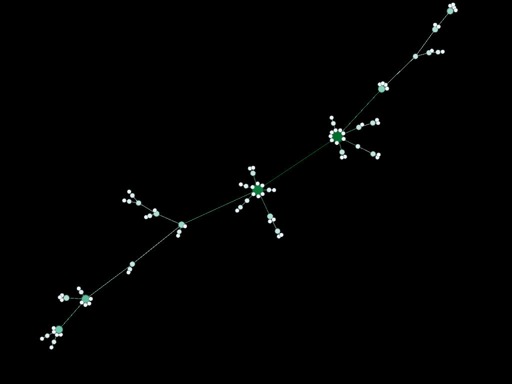
For example, Model 1 (below) started with 1 node and 1 node was added over 99 time steps and at each time step 1 attachment was made to one of the existing nodes. The ending network possesses 100 nodes and 99 total undirected attachments.
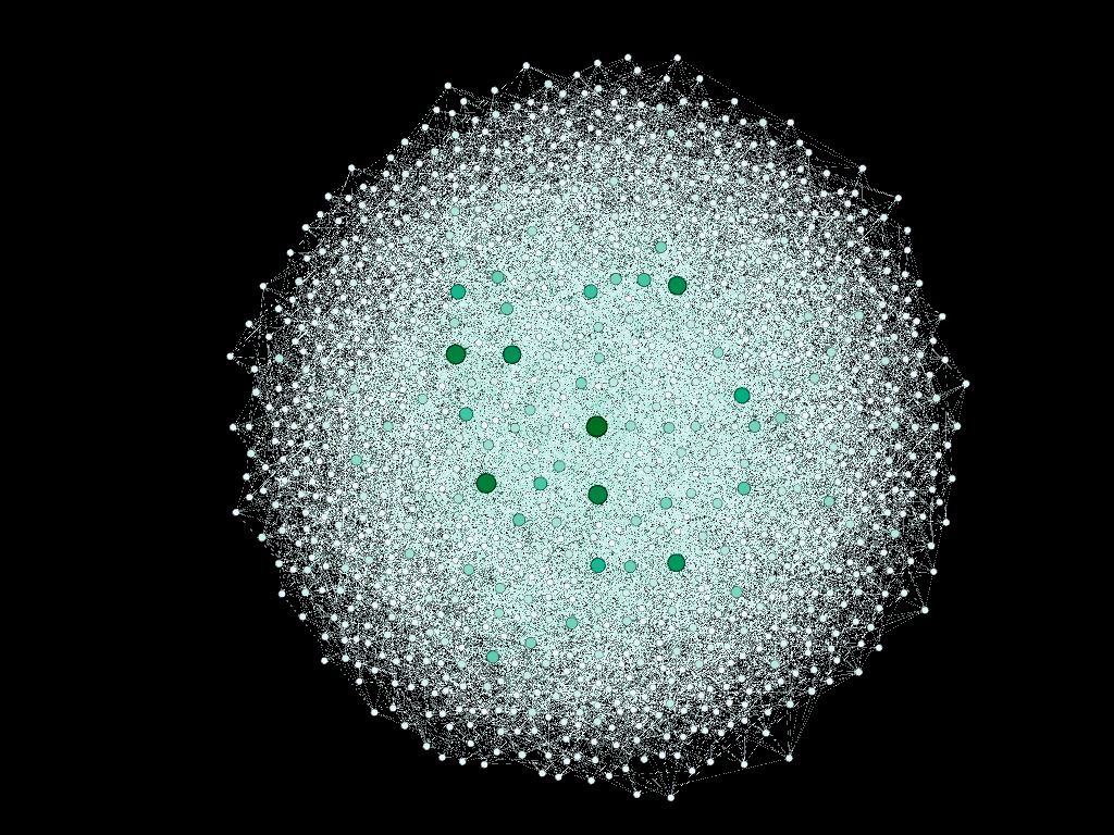
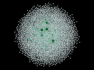
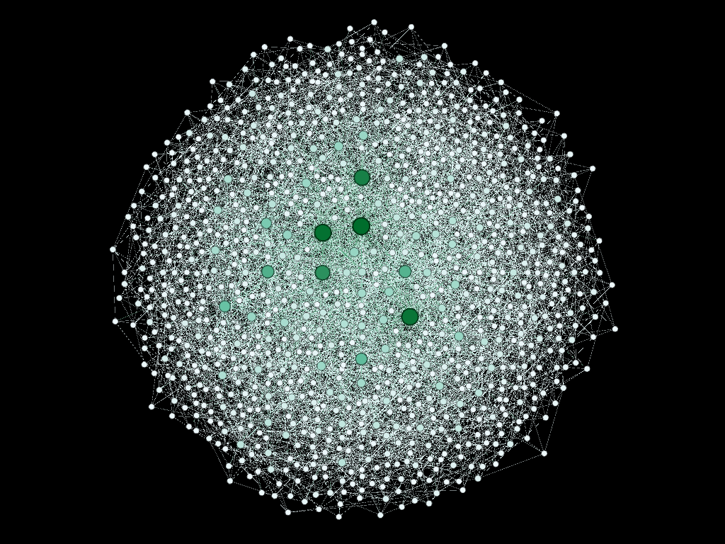
Similarly, Model 8 (below) started with 10 fully connected nodes and 10 nodes were added at each of 99 time steps and at each time step each new node made 10 new attachments to 10 randomly selected existing nodes. The ending network possesses 1000 nodes and 9945 undirected attachments.
For reference, a fully connected network consisting of 100 nodes would have 4950 undirected attachments and a fully connected network consisting of 1000 nodes would have 499,500 undirected attachments.
Network Statistics
As mentioned, we created eight randomly generated network models, four resulting in 100 nodes each and four resulting in 1000 each. The networks are considered to be undirected.
The table below presents some basic statistics for each model. As you can see, network density (the ratio of nodes to connections) is on the low end of the spectrum, ranging from 2% to 20% for Models 1 - 4 and 0.05% to 2% for Models 5 - 8. A completely connected network possesses a density of 100%.
The Average Degree is the average number of connections each node possess. The network Diameter is the maximum number of connections it takes to traverse from any one node to another across the network. The Clustering Coefficient measures the degree of connectedness within the network, different from density, but rather is a measure of how many of your friends are friends.
| Model | Agents | Avg. Degree | Diameter | Density | Clustering Coef. |
|---|---|---|---|---|---|
| M1 | 100 | 2 | 12 | 2% | 0.0 |
| M2 | 100 | 4 | 6 | 4% | 0.17 |
| M3 | 100 | 10 | 3 | 10% | 0.22 |
| M4 | 100 | 19 | 3 | 20% | 0.35 |
| M5 | 1000 | 2 | 19 | 0.05% | 0.0 |
| M6 | 1000 | 4 | 7 | 0.8% | 0.03 |
| M7 | 1000 | 10 | 5 | 1% | 0.05 |
| M8 | 1000 | 20 | 4 | 2% | 0.07 |
Note also that by continuing the PA process to 1000 nodes, versus 100 nodes, produced much less dense networks while retaining similar Degree and Diameter measures.
Network Visualizations
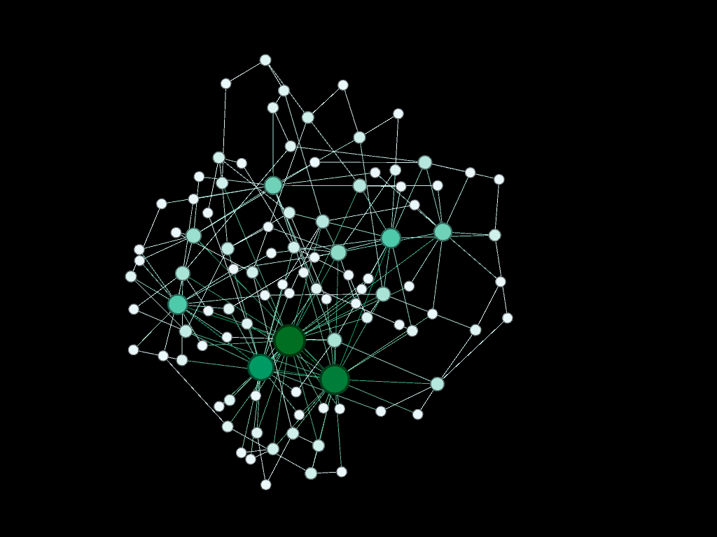
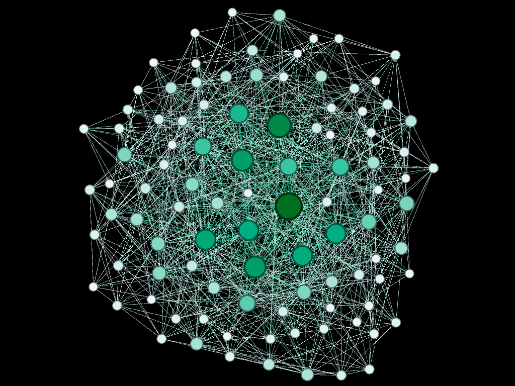
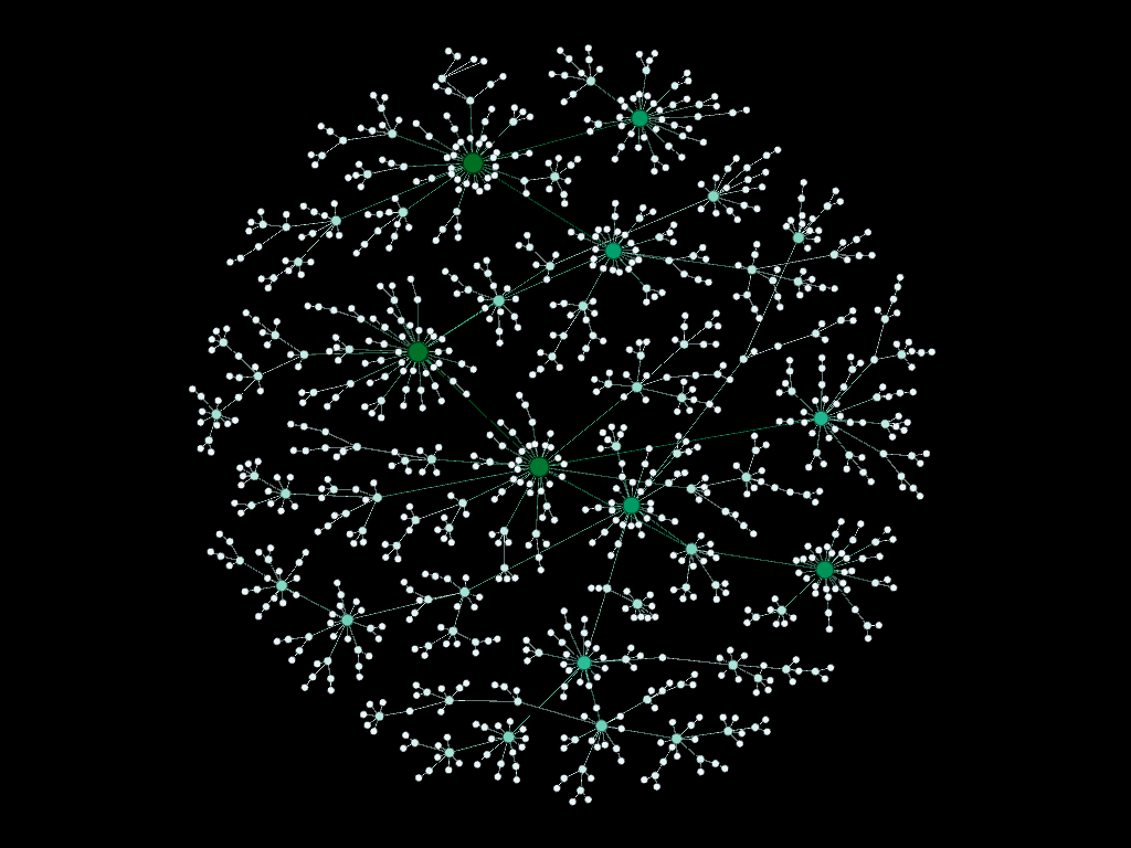
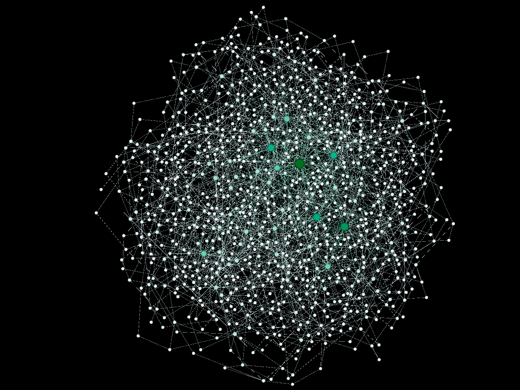
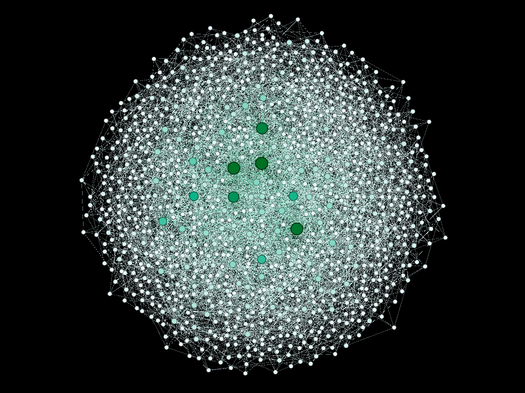
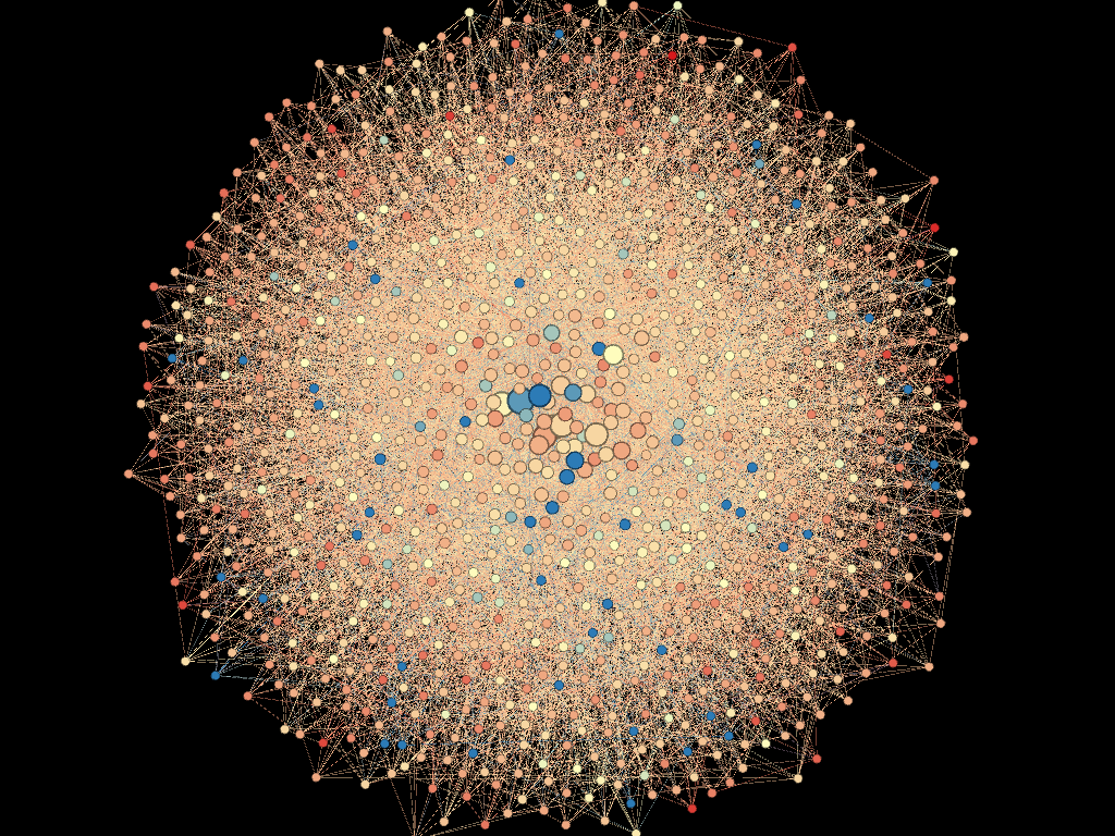
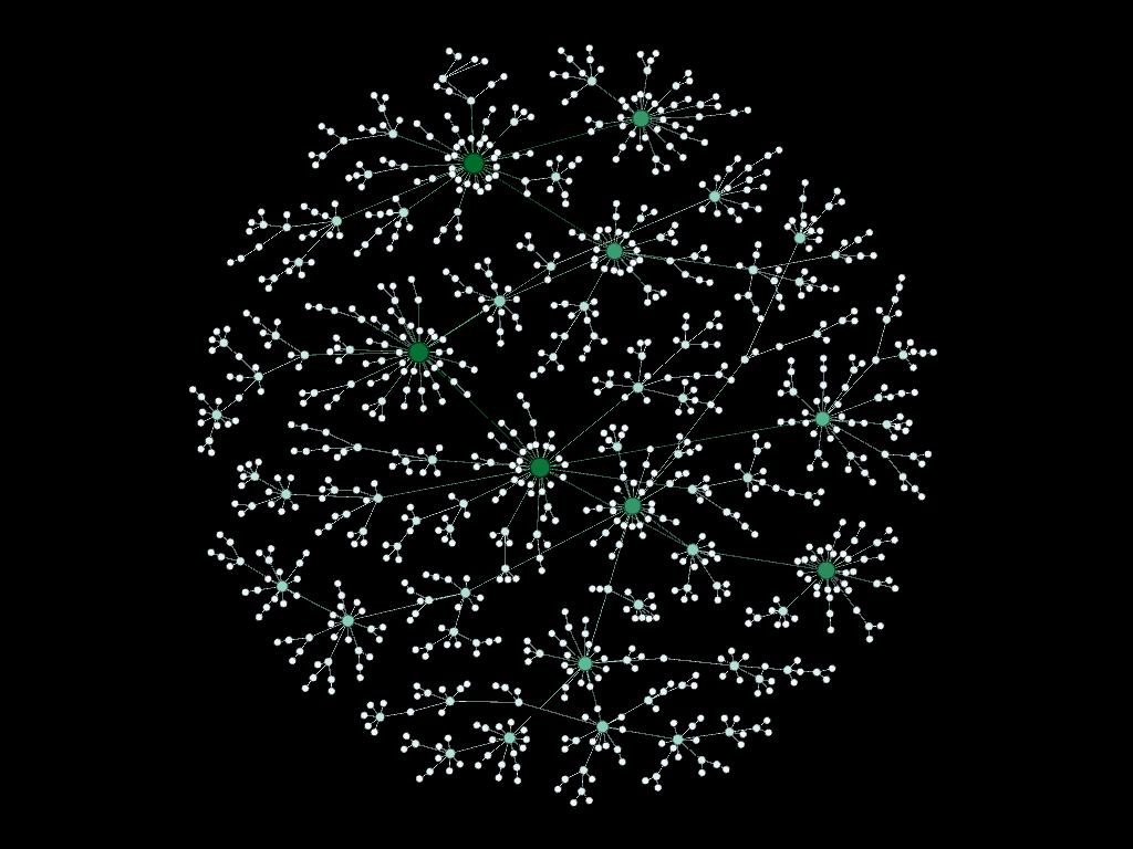
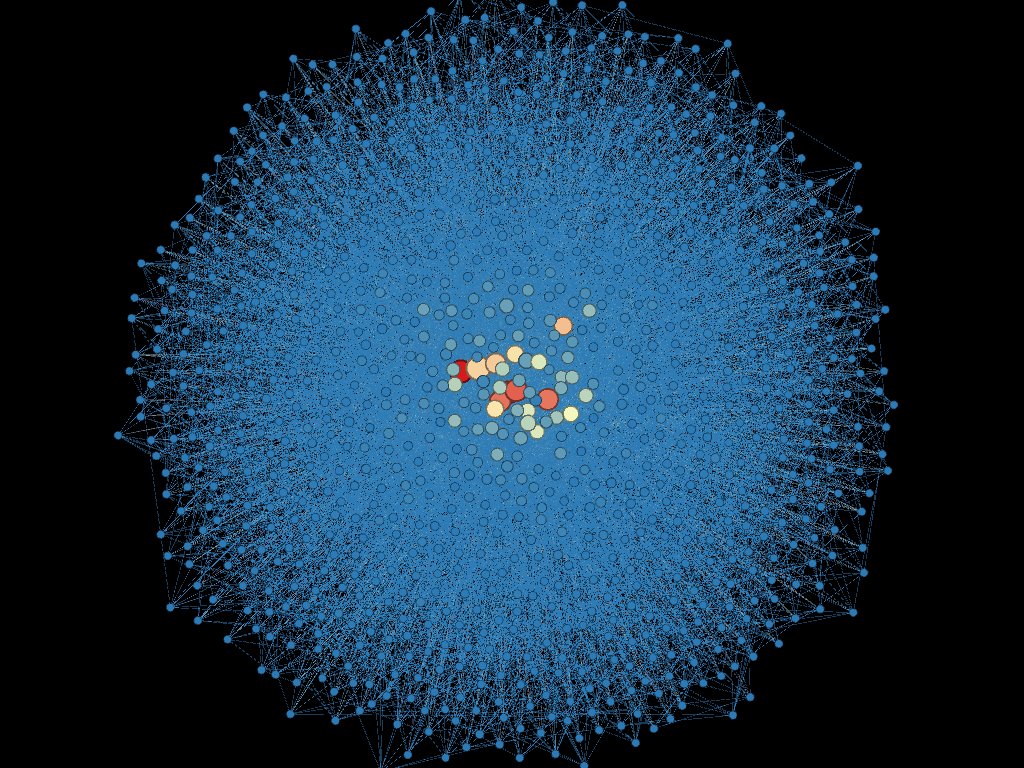
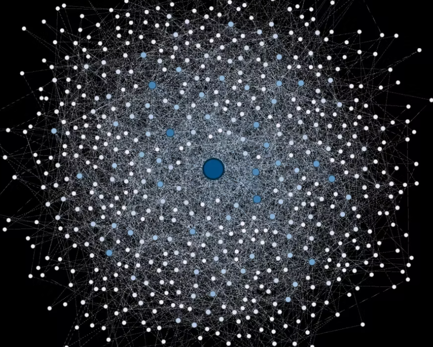
Statistics are important, but it's more fun to see what the networks actually look like. Below a diagram of each network is presented. The size and color of the each node is proportional to the number of connections each node possesses (smaller, whiter nodes possess fewer connections, larger, greener nodes possess more connections).
Note again, given the network generation processes, the nodes with more connections will typically be the "older" nodes on the network.
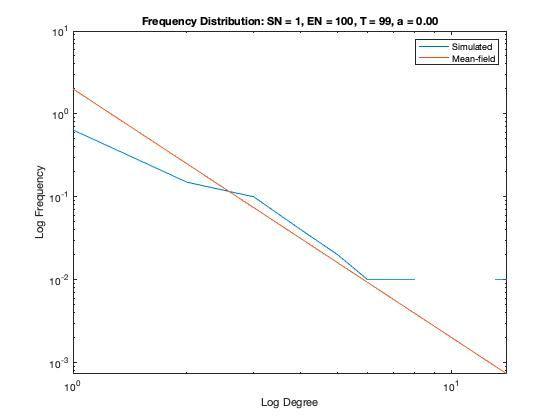
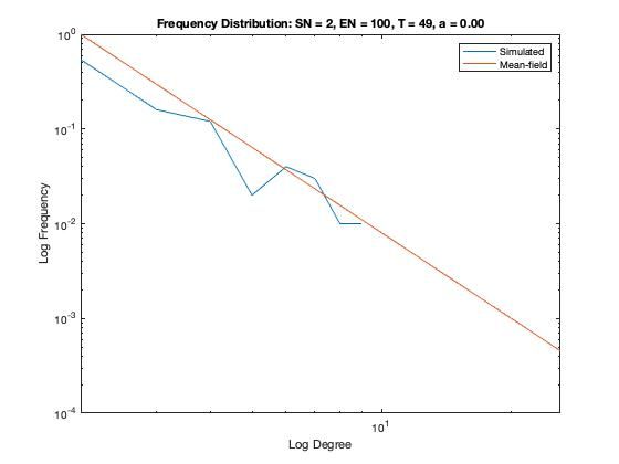
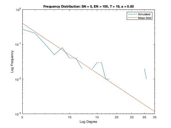
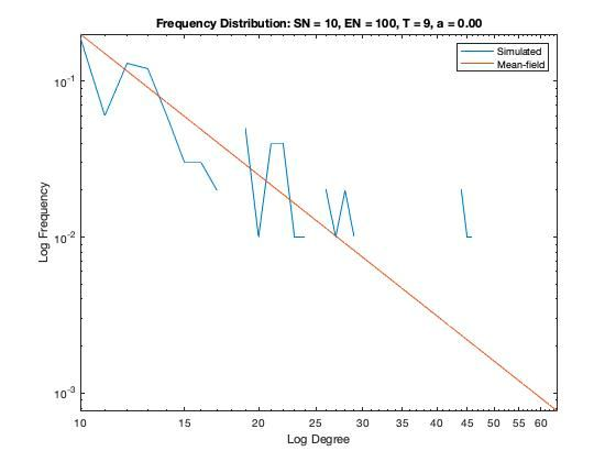
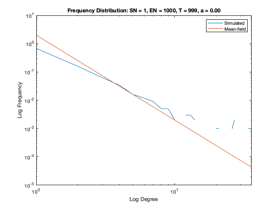
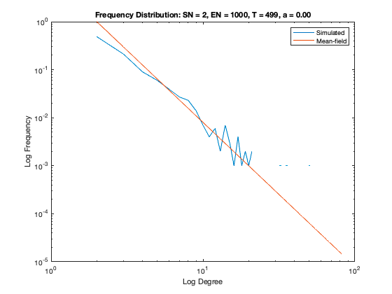
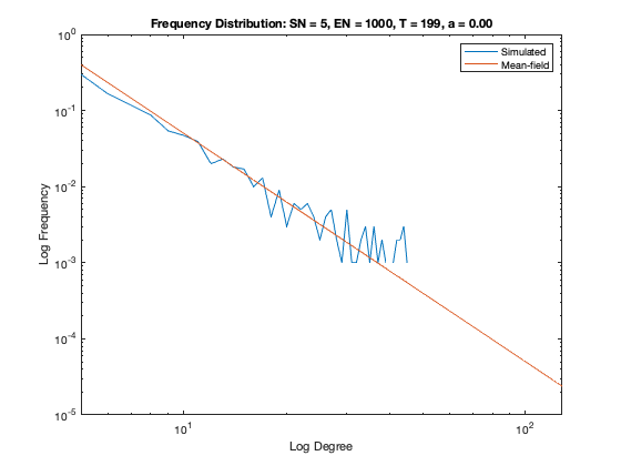
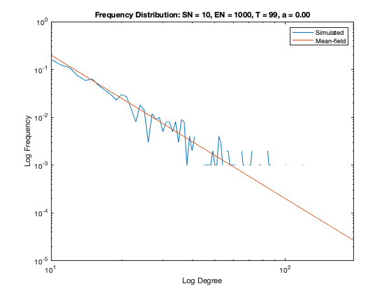
In addition to a visualization of each network model we plot the resulting degree distribution against its theoretical mean-field equivalent. We see a good correspondence between the simulated degree distribution and its mean-field equivalent, providing assurance the algorithm is functioning as intended.
Some nomenclature: SN = Starting Node Number, EN = Ending Node Number, T = Number of Time Steps. For example, Model 1 started with 1 node (SN=1), added one agent and one attachment for 99 time steps (T=99) creating 100 nodes total (EN=100).
Model 1 - Density = 2%
Model 2 - Density = 4%
Model 3 - Density = 10%
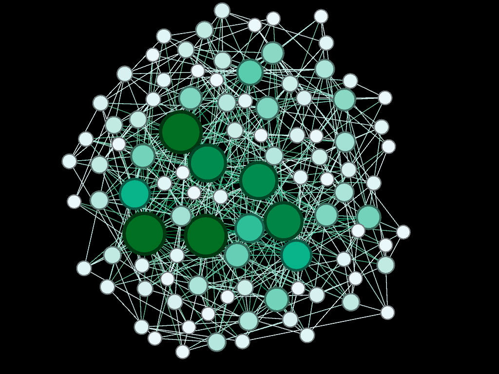
Model 4 - Density = 20%
Model 5 - Density = 0.05%
Model 6 - Density = 0.80%
Model 7 - Density = 1%
Model 8 - Density = 2%
References
Social and Economic Networks by Matthew O. Jackson, Princeton University Press, 2010